Decomposition of tensor tensor
Artificial intelligence, deep learning, convolutional neural network, reinforcement learning. These are revolutionary advances in the field of machine learning, which make many impossible tasks become possible. Despite these advantages, there are also some disadvantages and limitations. For example, because neural networks need a large number of training sets, it is easy to lead to over fitting. These algorithms are usually designed for specific tasks, and their capabilities can not be well transplanted to other tasks
One of the main challenges of computer vision is the amount of data involved: an image is usually represented as a matrix with millions of elements, while video contains thousands of such images. In addition, noise often appears in this kind of data. Therefore, unsupervised learning method which can reduce the dimension of data is a necessary magic weapon to improve many algorithms.
In view of this, tensor decomposition is very useful in the application of high-dimensional data. Using Python to implement tensor decomposition to analyze video can get important information of data, which can be used as preprocessing of other methods
High dimensional data
High dimensional data analysis involves a set of problems, one of which is that the number of features is larger than the number of data. In many applications (such as regression), this can lead to speed and model learning problems, such as over fitting or even unable to generate models. This is common in computer vision, materials science and even business, because too much data is captured on the Internet
One of the solutions is to find the low dimensional representation of the data and use it as the training observation in the model, because dimension reduction can alleviate the above problems. The lower dimensional space usually contains most of the information of the original data, so the reduced dimensional data is enough to replace the original data. Spline, regularization and tensor decomposition are examples of this method. Let’s study the latter method and practice one of its applications.
Project 3D data onto 2D plane, image source: May Morrison.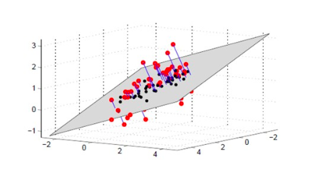
Mathematical concepts
The core concept of this paper is tensor
The number is a 0-dimensional tensor
A vector is a one-dimensional tensor
A matrix is a two-dimensional tensor
in addition, it directly refers to the dimension of tensor
This data structure is particularly useful for storing images or videos. In the traditional
RGB model
In [1] , a single image can be represented by a three-dimensional tensor
each color channel (red, green, blue) has its own matrix, and the value of a given pixel in the matrix encodes the intensity of the color channel
Each pixel has (x, y) coordinates in the matrix, and the size of the matrix depends on the resolution of the image
The representation of 3D tensor. For images, , and And It represents the resolution of the image. Image sources: Kolda, Tamara g. and Brett W. Bader.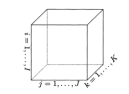
Further, a video is just a series of frames, each of which is an image. It makes it difficult to visualize, but it can be stored in 4D tensor: three dimensions are used to store a single frame, and the fourth dimension is used to encode the passage of time
Each slice is a 3D tensor representing a certain frame, and there are multiple slices along the time axis. Image source: kamran paynabar.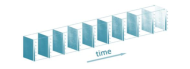
To be more specific, let’s take a 60 second video with 60 frames per second (frames per second) and a resolution of 800×600 as an example. The video can be stored in 800x600x3600 tensor. So it’s going to have five billion elements! That’s too much for building a reliable model. That’s why we need tensor decomposition
There are many literatures about tensor decomposition, and I recommend Kolda and balder’s
overview
[2]。 In particular, Tucker decomposition has many applications, such as tensor regression
Objectives
[3] or
forecast
[4] variable. The key point is that it allows the extraction of a kernel tensor, a compressed version of the original data. If this reminds you of PCA, that’s right: one of the steps in Tucker decomposition is actually an extension of SVD, that is, SVD
high order singular value decomposition .
Existing algorithms allow the extraction of kernel tensor and decomposition matrix (not used in our application). The super parameter is rank n. The main idea is that the higher the n value is, the more accurate the decomposition is. Rank n also determines the size of the kernel tensor. If n is small, the reconstructed tensor may not exactly match the original tensor, but the lower the data dimension is, the trade-off depends on the current application.
A. B and C are decomposition matrices, and G is kernel tensor whose dimension is specified by n. Image sources: Kolda, Tamara g. and Brett W. Bader.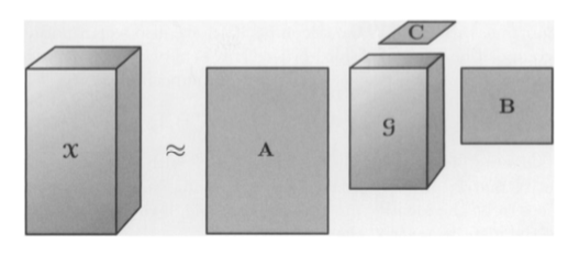
It is very useful to extract this kernel tensor, which will be seen in the following practical application examples.
Application
As an example of a toy, I captured three 10 second videos on my mobile phone:
My favorite cafe terrace
Parking lot
Cars on the freeway during the afternoon commute
I uploaded them and notbook code to GitHub. The main purpose is to determine whether we can strictly rank potential video pairs according to the similarity under the premise that parking lots and commuting videos are the most similar.
Before analyzing, use opencv Python library to load and process this data. The steps are as follows,
Create videocapture objects and extract the number of frames for each object
I use a shorter video to truncate the other two for better comparison
#Importlibraries
importcv2
importnumpyasnp
importrandom
importtensorlyastl
fromtensorly.decompositionimporttucker
#CreateVideoCaptureobjects
parking_lot=cv2.VideoCapture('parking_lot.MOV')
patio=cv2.VideoCapture('patio.MOV')
commute=cv2.VideoCapture('commute.MOV')
#Getnumberofframesineachvideo
parking_lot_frames=int(parking_lot.get(cv2.CAP_PROP_FRAME_COUNT))
patio_frames=int(patio.get(cv2.CAP_PROP_FRAME_COUNT))
commute_frames=int(commute.get(cv2.CAP_PROP_FRAME_COUNT))
Randomly sample 50 frames from these tensors to speed up subsequent operations
#Settheseedforreproducibility
random.seed(42)
random_frames=random.sample(range(0,commute_frames),50)
#Usetheserandomframestosubsetthetensors
subset_parking_lot=parking_lot_tensor[random_frames,:,:,:]
subset_patio=patio_tensor[random_frames,:,:,:]
subset_commute=commute_tensor[random_frames,:,:,:]
#Convertthreetensorstodouble
subset_parking_lot=subset_parking_lot.astype('d')
subset_patio=subset_patio.astype('d')
subset_commute=subset_commute.astype('d')
After completing these steps, we get three 50x1080x1920x3 tensors.
Results
To determine how similar these videos are, we can rank them. The L2 norm of the difference between two tensors is a common measure of similarity. The smaller the value is, the higher the similarity is. In mathematics, the norm of tensor can be
Each Represents a given dimension, Is a given element.
Therefore, the norm of difference is similar to Euclidean distance
The result of this operation using complete tensor is not satisfactory.
#Parkingandpatio
parking_patio_naive_diff=tl.norm(subset_parking_lot-subset_patio)
#Parkingandcommute
parking_commute_naive_diff=tl.norm(subset_parking_lot-subset_commute)
#Patioandcommute
patio_commute_naive_diff=tl.norm(subset_patio-subset_commute)
Look at the similarities
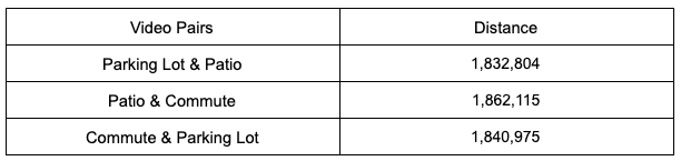
Not only is there no clear ranking between the two videos, but the parking lot and terrace videos seem to be the most similar, in sharp contrast to the original assumption
Well, let’s see if Tucker decomposition can improve the results.
Tensorly library makes it relatively easy to decompose tensors, although it’s a bit slow: all we need is tensors and their rank n. Although AIC criterion is a common method to find the optimal value of this parameter, it is not necessary to achieve the optimal value in this particular case, because the purpose is to compare. We need all three variables to have the same rank n. Therefore, we choose n-rank = [2, 2, 2, 2], which is a good tradeoff between accuracy and speed. By the way, n-rank = [5,5,5,5] exceeds the function of LAPACK (low level linear algebra package), which also shows that these methods are computationally expensive.
After extracting the kernel tensor, the same comparison can be made.
#Getcoretensorfortheparkinglotvideo
core_parking_lot,factors_parking_lot=tucker(subset_parking_lot,ranks=[2,2,2,2])
#Getcoretensorforthepatiovideo
core_patio,factors_patio=tucker(subset_patio,ranks=[2,2,2,2])
#Getcoretensorforthecommutevideo
core_commute,factors_commute=tucker(subset_commute,ranks=[2,2,2,2])
#Comparecoreparkinglotandpatio
parking_patio_diff=tl.norm(core_parking_lot-core_patio)
int(parking_patio_diff)
#Comparecoreparkinglotandcommute
parking_commute_diff=tl.norm(core_parking_lot-core_commute)
int(parking_commute_diff)
#Comparecorepatioandcommute
patio_commute_diff=tl.norm(core_patio-core_commute)
int(patio_commute_diff)
Look at the similarity
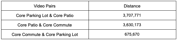
These results make sense: Although terrace videos are different from parking and commuting videos, the latter two videos are closer to an order of magnitude.
Conclusion
In this article, I show how unsupervised learning methods provide insight into data. Only when the dimension is reduced by Tucker decomposition to extract the kernel tensor from the video, can the comparison be meaningful. We confirm that the parking lot is the most similar to the commuter video
As video becomes more and more popular data source, this technology has many potential applications. The first thought (due to my passion for TV and how the video streaming service uses data) is to improve the existing recommendation system by checking the similarities between some key scenes of the trailer or movie/TV program. The second is materials science, in which the heated metal can be classified according to the similarity between the infrared video and the benchmark. In order to make these methods fully scalable, we should solve the computational cost: on my computer, Tucker decomposition speed is very slow, although only three 10s small videos. Parallelization is a potential way to speed up processing.
In addition to these direct applications, the technique can also be combined with some of the methods introduced in the introduction. Using the core tensor instead of the whole image or video as the training points in the neural network can help to solve the over fitting problem and speed up the training speed, so as to enhance the method by solving these two main problems.
In this paper, through an example, let us initially understand the tensor decomposition tool, and master the actual usage through the code. Please click here [5] for children’s shoes that need to download this code to consolidate understanding. If you want to have a deep understanding of tensor decomposition, please read the references. The detailed interpretation of the theoretical knowledge of tensor decomposition will be introduced later
References
[1]
RGB model https://en.wikipedia.org/wiki/RGB_ color_ model
[2]
summary: http://www.kolda.net/publication/TensorReview.pdf
[3]
Objective: https://arxiv.org/abs/1807.10278
[4]
prediction: https://arxiv.org/pdf/1706.03423.pdf
[5]
code: https://github.com/celestinhermez/video-analysis-tensor-decomposition
[6]
English link: https://towardsdatascience.com/video-analysis-with-tensor-decomposition-in-python-3a1fe088831c
– END –
this article is shared by WeChat official account – machine learning and Mathematics (Mathinside2016).
Similar Posts:
- tf.nn.top_k(input, k, name=None) & tf.nn.in_top_k(predictions, targets, k, name=None)
- Python TypeError: softmax() got an unexpected keyword argument ‘axis’
- [Solved] Tensorflow TypeError: Fetch argument array has invalid type ‘numpy.ndarry’
- Solutions to errors encountered by Python
- [Solved] PyTorch error: TypeError: ‘builtin_function_or_method‘ object is unsubscriptable
- Reasoning With Neural Tensor Networks For Knowledge Base Completion-paper
- What are hyperparameters in machine learning?
- Image data type conversion uint8 and double in MATLAB
- xxx/labelKeypoint/utils/qt.py:81: RuntimeWarning: invalid value encountered in double_scalars
- LinAlgError: Last 2 dimensions of the array must be square